It’s often useful to visually understand how one statistic relates to another. For example, to see how rental apartment area affects its monthly price. The first visualization that would come to my mind is scatter plot, and I argue that scatter plot is not descriptive enough to offer good understanding of the simple case of two 1d statistics. I propose a rich boxplot visualization that gives better overview of the correlation to the reader.
Example data
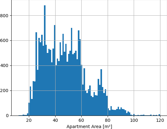
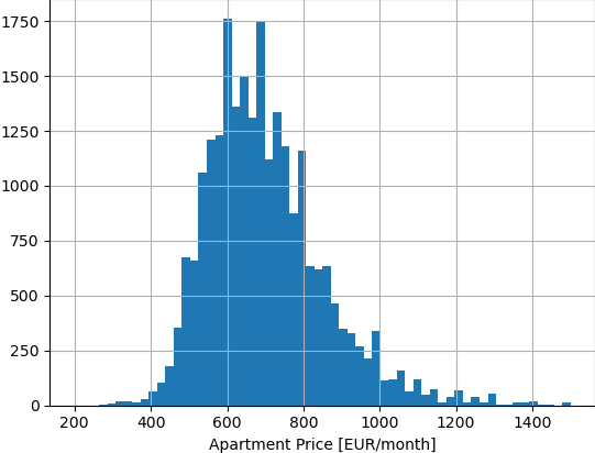
Given about 24000 rental ads for apartments in Tampere, Finland in the last 3 years, perhaps in a DataFrame with two columns “area” and “price”, these are the distributions of apartment size in square meters, and apartment price in EUR per month.
 |
| 
You can see that the histogram of apartment size is peaky, developers stick to certain apartment sizes. As there are many new high blocks of flats, the apartment sizes are the same for apartments above and below in the same block. The peaks can be seen as popular apartment sizes in Tampere. There’s 25 m², 32 m², 39 m², 45 m², 52 m², 59 m² and then 75 m².
The price is less peaky and more “naturally” (normally) distributed. Median is 680 EUR, but there is another peak around 600.
I have already removed some outlier categories, for example:
- short-term hotel-like apartments (Forenom), where 25 m² studio comes to 1200 EUR/month
- single rooms - listings of area <20 m²
- listings out of sensible range for price and area
Scatter Plot
Now it would be good to see how the apartment size relates to the rental price. Let’s scatter plot. Scatter plot is a 2d plot where each data point (row in our dataframe) is displayed on [x,y] coordinates [area,price]. This is a scatter plot of area and price of rental apartments in Tampere:
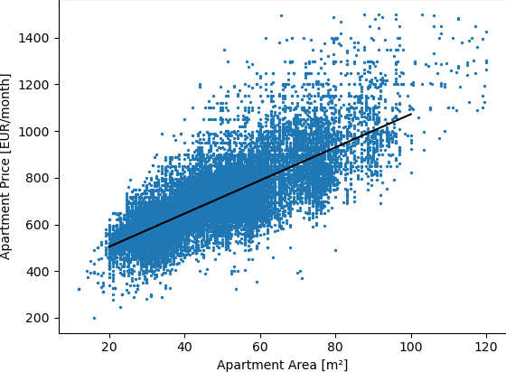
The blue dots are the datapoints, and the black line is a linear function fitted from all the datapoints. The line (linear function) says that, given no data but the apartment size, you can estimate rental price of an apartment in Tampere by solving
Price [EUR] = 362 + 7.1 * Size [m²]
.. so for 50 m² we get 717 EUR, which seems about right by looking at the scatter plot. It would be interesting to see what those coefficients (362 and 7.1) would be for other cities in Finland.
We can get a good feel of the relationship between the two distributions from the scatter plot and fitted linear function. However, coming from the histograms, we lose information about local density of the data. We don’t know how strong is the evidence for particular apartment size (or size interval). The linear function is surely more precise for median-sized apartments than for large ones (more than 100 m²) because those are much less common. We also have very limited information about how much the price spreads for a particular apartment size.
Even though we only investigate apartment size as a factor of price, it’s also interesting to see to what extent is the the price affected by the other features (year built, location, amenities, ..). We can get the idea by examining how much the price varies for a given size interval, e.g. what is the price range for the most common half of apartments between 49 and 51 m². Looking at the scatter plot, I could guess that it will be from ~600 to ~800, but I have no means to qualitatively compare this guess to other size ranges.
Furthermore, a linear function will not have good information value for non-linear relationships, e.g. age of an apartment - very old (1950s) and very new (2010s) apartments will be more expensive than apartments built in the middle of the era (1980s).
Rich boxplot
The variance can be explained by using a boxplot. For some reason, boxplots are mostly used in scientific papers, and display dependency of numeric variable on a categorical variable, think sth like petal lenghts of species of the Iris flower.
In order to transform the scatter plot to be more informative, I decided to bin the control variable (size), and display the median and the 0.25 and 0.75 quantiles of prices in the bin. It’s not too hard to compute that, for apartments between 49 and 51 m², there is 1208 datapoints, the median price is 710 cheapest 25% of the apartments are below 650 (0.25 quantile) and the cheapest 75% of the apartments are below 780 (0.75 quantile). This means that the most common half of 49-51 m² apartments in Tampere are between 650 and 780 EUR per month.
Let’s take the 2D space from the scatter plot and imagine a rectangle with vertical edges on the apartment size interval bounds, and horizontal edges on the 25% and 75% percentile prices, with a dot on the median price level. for the example from previous paragraph, it would be a rectangle between points [49,650], [51,650], [51, 780] and [49, 780], with a dot on [50, 715]. If we divide all the size range into intervals, and then transform all of them into such rectangles, the plot will look like this:
You can hover over a rectangle and the tooltip will show parameters of the bin. I added histograms for both of the statistics (above and on the left), and I adjust intensity of the bin based on how many samples are in it. the darker the bin, the more samples it contain. I don’t show borders of the size interval, but rather the middle value from the interval. The width of the bin/interval is not important, and can be roughly estimated from the mid-value distance.
The rich boxplot will show how much the price values disperse based on the apartment size. It doesn’t only report the relationship between the variables but also the quality of the data in the range.